Retrieving a Layer by Bounding Box • firex

This vignette shows the simplest data retrieval workflow: request one layer for one rectangular area of interest. get_layer() opens the hosted Cloud Optimized GeoTIFF (COG) through GDAL and uses range requests, so the user does not need to download the full raster file.

Setup

library(firex)
library(terra)

The Basic Call

get_layer() takes a layer ID, an aoi argument, and for numeric bounding boxes an explicit aoi_crs. Supply the bounding box as c(xmin, ymin, xmax, ymax). The function checks overlap against the layer extent and returns a terra raster in the COG native projection.

# Santa Barbara County, CA in WGS84
sb <- c(-120.7, 34.4, -119.4, 35.1)

wri <- get_layer("WRI_score", aoi = sb, aoi_crs = "EPSG:4326")
wri
#> class       : SpatRaster
#> dimensions  : 482, 756, 1  (nrow, ncol, nlyr)
#> resolution  : 90, 90  (x, y)
#> coord. ref. : NAD83 / Conus Albers (EPSG:5070)
#> name        : WRI_score

Plotting the Result

plot(
  wri,
  main = "WRI Score -- Santa Barbara County",
  col = hcl.colors(100, "YlOrRd", rev = TRUE)
)

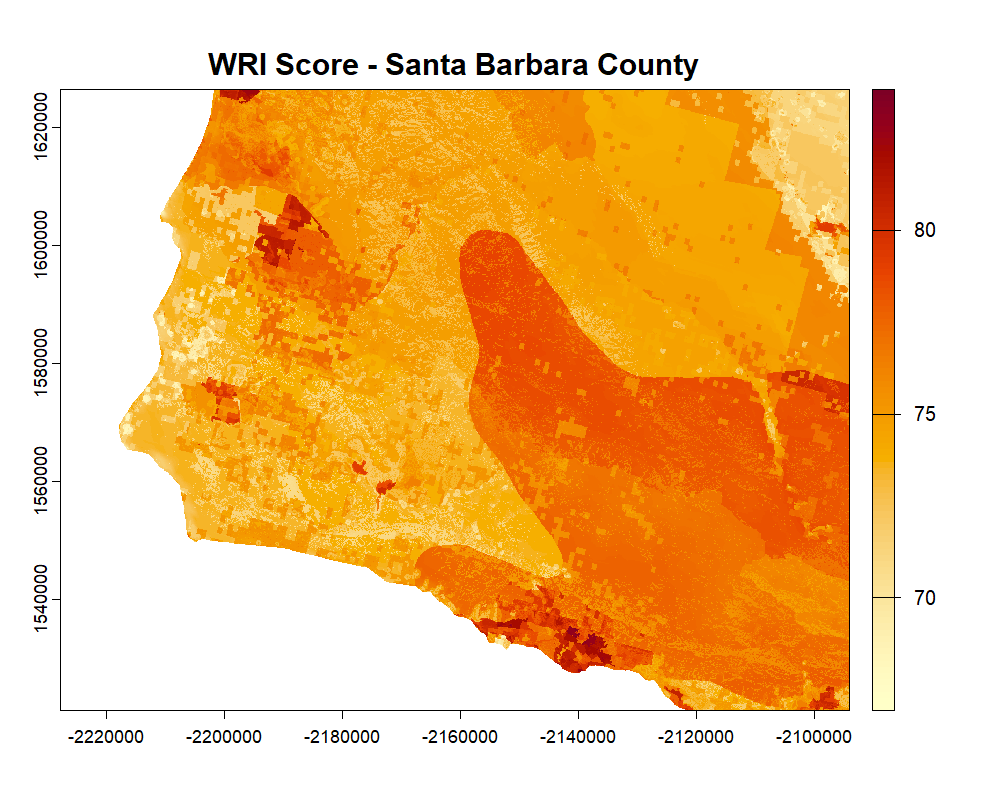
Figure 4. WRI score for a bounding box over Santa Barbara County, CA, returned by get_layer(). Darker red values indicate higher WRI score values.

Working With the Result

Because get_layer() returns a standard SpatRaster, the full terra ecosystem is immediately available for analysis:

# Summary statistics
global(wri, fun = c("mean", "sd", "min", "max"), na.rm = TRUE)
#>    mean    sd  min   max
#>   0.531 0.112 0.18 0.894

# Write to disk as a GeoTIFF
writeRaster(wri, "wri_score_sb.tif")

# Reproject to WGS84 for export to other tools
wri_wgs84 <- project(wri, "EPSG:4326")

CRS Shorthand

aoi_crs accepts any format that terra recognizes: an integer EPSG code, a character string, or a PROJ or WKT string. These are all equivalent:

get_layer("WRI_score", aoi = sb, aoi_crs = 4326)
get_layer("WRI_score", aoi = sb, aoi_crs = "EPSG:4326")
get_layer("WRI_score", aoi = sb, aoi_crs = "WGS84")

Retrieving Multiple Layers for the Same Area

Use lapply() to iterate over a vector of layer IDs. All layers share the same extent and resolution once retrieved, so the results can be stacked directly with terra::c():

water_ids <- subset(
  wri_overview_df(),
  wri_domain == "water" & data_type == "aggregate"
)$id

water_layers <- lapply(
  water_ids,
  get_layer,
  aoi = sb,
  aoi_crs = "EPSG:4326"
)

names(water_layers) <- water_ids

stack <- do.call(c, water_layers)
plot(stack, col = hcl.colors(100, "YlOrRd", rev = TRUE))

Extent Overlap and Error Handling

If the bounding box extends partly outside the COG coverage area, get_layer() returns the overlapping portion and issues a warning naming the sides that overflowed:

wri_big <- get_layer(
  "WRI_score",
  aoi = c(-130, 30, -55, 55),
  aoi_crs = "EPSG:4326"
)
#> Warning: Requested bbox extends outside the layer extent to the east.

If the bounding box falls entirely outside the covered area, the function stops with an informative error before making any network request:

tryCatch(
  get_layer(
    "WRI_score",
    aoi = c(-80, -90, -60, -70),
    aoi_crs = "EPSG:4326"
  ),
  error = function(e) message("Error: ", conditionMessage(e))
)
#> Error: Requested bbox does not overlap the layer extent.

Use a polygon boundary in place of a rectangular bounding box when you already have a study area saved as a spatial object or file.